Vision-Language-Action (VLA) Robotic Arm Control System
1. Introduction
This document describes the complete technical architecture of a Vision-Language-Action (VLA) robotic arm control system built for the Niryo robotic arm, simulated in CoppeliaSim. The system enables a user to type a natural language instruction such as "pick the red cube and place it in square" and have the robot arm autonomously execute the described pick-and-place task.
The system is composed of three decoupled layers:
- A local YOLO-based vision layer that detects and localises objects in the scene using bounding boxes.
- A behavioural cloning (BC) neural network that learns to produce smooth joint-space trajectories conditioned on visual observations and a goal end-effector pose.
- A classical inverse-kinematics (IK) execution layer inside CoppeliaSim that converts predicted poses into physical joint commands.
2. System Architecture
Key Design Principle
The core design is based on a fully offline, self-contained system and YOLO colour detection, ensuring no external API dependence or usage limits. The neural network's sole function is visual servoing: determining the next pose based on the current and target positions.
Layer 1 — Language Understanding
The reasoning tasks were successfully executed and analyzed using the locally hosted Ollama 3 model. The user's free-form instruction is parsed into a structured goal: an object to pick and a destination zone. This step requires no cloud API — inference runs entirely on local hardware.
Layer 2 — Goal Pose Computation (Classical Geometry)
The model is trained on a seven-valued action space. The YOLO model extracts image-space coordinates, which are then projected to simulation-space coordinates, giving the arm spatial awareness of both the target object and the destination zone.
Action vector: [x, y, z, pitch, roll, yaw, gripper]
| Dimension | Physical Meaning | Range |
|---|---|---|
| 0 — x | End-effector X position (metres) | -0.19 to +0.19 |
| 1 — y | End-effector Y position (metres) | +0.25 to +0.50 |
| 2 — z | End-effector Z position (metres) | -0.05 to +0.50 |
| 3 — pitch | Wrist pitch angle (radians) | -π/2 to +π/4 |
| 4 — roll | Wrist roll angle (radians) | -π to +π |
| 5 — yaw | Wrist yaw angle (radians) | -20° to +20° |
| 6 — gripper | Gripper open/close target | 0.0 (open) / 1.0 (closed) |
Layer 3 — Trajectory Generation (Neural Network)
This is what the neural network actually learns. Given: (a) the current camera images, (b) the current robot state, and (c) the goal end-effector pose — predict the next end-effector pose the arm should move toward.
This is called behavioural cloning. We recorded 100 expert demonstrations of a human teleoperating the arm to complete various pick-and-place tasks. The network watches those demonstrations and learns the pattern: what smooth approach trajectories look like, when to lower the gripper, when to close it, how to transport without collision, how to descend and release at the destination.
DATA_GENERATION -> NORMALIZATION -> TRAINING -> INTERFACE
SCENE -> IK SOLVER -> POS[ACTION VECTOR]
3. Algorithms
3.1 Raw Dataset Structure
Each demonstration trajectory is stored as a folder inside dataset/. A trajectory captures one complete pick-and-place task from start to finish, recorded at 10 Hz.
Folder structure:
dataset/
└── traj_001/
    ├── top_images/       000000.png 000001.png ... (top-down RGB frames)
    ├── wrist_images/     000000.png 000001.png ... (wrist RGB frames)
    ├── states.npy        shape (N, 13) — robot state at each timestep
    └── instruction.txt   e.g. 'pick the red cube and place it in zone b'
3.2 Data Normalisation
Before training, all action values are normalised to the [-1, +1] range using per-dimension min/max statistics computed across the full dataset. This prevents any single dimension (e.g. position in metres) from dominating the loss. The same statistics are stored and applied at inference time to convert network outputs back to real-world units.
# Normalise a raw action vector to [-1, +1]
action_norm = 2.0 * (action - action_min) / (action_max - action_min) - 1.0

# Denormalise at inference time
action_raw = (action_norm + 1.0) / 2.0 * (action_max - action_min) + action_min
3.3 Neural Network Architecture (vla_model.py)
NiryoVLA is a multi-modal behavioural cloning network. It fuses four input streams — two camera images, the robot state, and the goal EE pose — through separate encoders, concatenates the feature vectors, and predicts the normalised 7D action for the current timestep.
3.3.1 Input Streams
| Input | Shape | Encoder |
|---|---|---|
| Top camera image | [B, 3, 224, 224] |
ResNet-18 → Linear(512, 256) |
| Wrist camera image | [B, 3, 224, 224] |
ResNet-18 → Linear(512, 256) |
| Robot state | [B, 13] |
MLP: 13→64→64 with ReLU |
| Goal EE pose | [B, 6] |
MLP: 6→32→32 with ReLU |
3.3.2 Architecture Diagram
Top Camera [B,3,224,224]   Wrist Camera [B,3,224,224]   State [B,13]   Goal [B,6]
       │                           │                         │               │
  ResNet-18 → 256d            ResNet-18 → 256d          MLP → 64d      MLP → 32d
       └───────────────────────────┴─────────────────────────┴───────────────┘
                                   Concatenate → [B, 608]
                          Fusion MLP: 608 → 256 → 128 → 7
                              (ReLU, Dropout 0.1, Tanh output)
                           Predicted Action → [B, 7] in [-1, +1]
3.3.3 Parameter Count
- Top ResNet-18 encoder: ~11.2 M
- Wrist ResNet-18 encoder: ~11.2 M
- State MLP (13→64→64): ~5,000
- Goal pose MLP (6→32→32): ~1,300
- Fusion MLP (608→256→128→7): ~189,000
Total: ~22.6 M parameters
3.4 Vision Detection System (vision_parser.py)
The vision parser replaces any external LLM API with a fully local, offline pipeline using YOLOv8 for object detection and HSV colour masking for object identification. Each frame from the top-down camera is passed through YOLOv8 to produce bounding boxes; the correct box is then selected by matching its dominant HSV colour to the colour named in the instruction (e.g. "red cube").
3.4.1 2D Bounding Box → 3D World Position
The 2D pixel centre of the selected bounding box is projected to a 3D world coordinate using a simple pinhole camera model. The camera is mounted directly above the table pointing straight down, so depth equals camera height minus object height above the table surface.
depth   = CAM_HEIGHT_M - (object_z - TABLE_Z)
x_cam   = (px - CX) * depth / focal_length
y_cam   = (py - CY) * depth / focal_length
world_x = table_centre_x + x_cam
world_y = -y_cam
world_z = TABLE_Z + object_height
Camera constants (CAM_WIDTH=512, CAM_HEIGHT=512, CAM_FOV_DEG=60, CAM_HEIGHT_M=1.2) must be matched to the CoppeliaSim vision sensor settings.
4. Outcome
4.1 Training Results
The graph below shows the Mean Squared Error (MSE) loss over 30 training epochs for the NiryoVLA model.
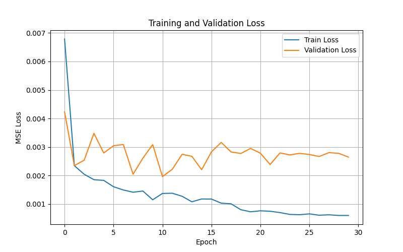
- X-Axis (Epoch): Represents one full pass of the demonstration dataset through the neural network.
- Y-Axis (MSE Loss): Measures the average squared difference between the robot's predicted 6D pose and the actual human demonstration. Lower values indicate predictions closer to expert behaviour.
- Blue Line (Train Loss): Shows the error on the 90% of data used to update network weights. It decreases steadily, reaching roughly 0.0006, confirming the network is successfully learning the training patterns.
- Orange Line (Validation Loss): Shows the error on the held-out 10%. It stabilises between 0.002 and 0.0035, indicating reasonable generalisation to unseen scenes.
4.2 YOLO Object Detection
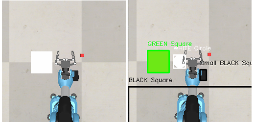
The image below shows a representative frame from the top-down camera with YOLOv8 bounding boxes overlaid. Each detected object is labelled with its class and confidence score; the HSV colour filter then selects the correct target based on the instruction.
4.3 GitHub Repository
GitHub Link: https://github.com/cyan-ide7/vla_arm.git